Disturbance
Disturbances comprise the following scenarios:
- fire events, which affect trees depending on their fire resistance
- landslide events, which create bare soil
In total, $N_D$ individuals of a cohort are dying due to disturbance induced mortality events.
Fire
The fire module in FORMIND is published in Fischer 2021. Fire is the primary disturbance process affecting the terrestrial biosphere (Pfeiffer et al. 2013). Especially wildfires affect species composition and vegetation structure in forests. They lead to a decrease of carbon storage and result in the emission of greenhouse gases. There is a long tradition in fire ecology to understand these processes and their interactions. Numerous methods were developed to estimate the disturbances due to fire events. Fire events are a complex distubances, which can be described by fire frequency, fire area and severity.
To understand the effect of fire on vegetation dynamics and vegetation structure, we developed the forest fire module ForFire, which is a combination of the ideas of wellestablished fire models (Gardner et al. 1999 Keane et al. 2004 Thonicke et al. 2001). External inputs to the ForFire module are the mean fire frequency per hectare and year ($\lambda$ in $[years]$), the mean fire size related to the investigated forest area ($\beta$ in $[\%]$) and the mean fire severity ($s_{fire}$ $[0-1]$). Fire events are implemented on the patch level, i.e. the smallest possible fire size has the size of one patch ($A_{patch}$), the biggest are considered are all patches of the simulation area.
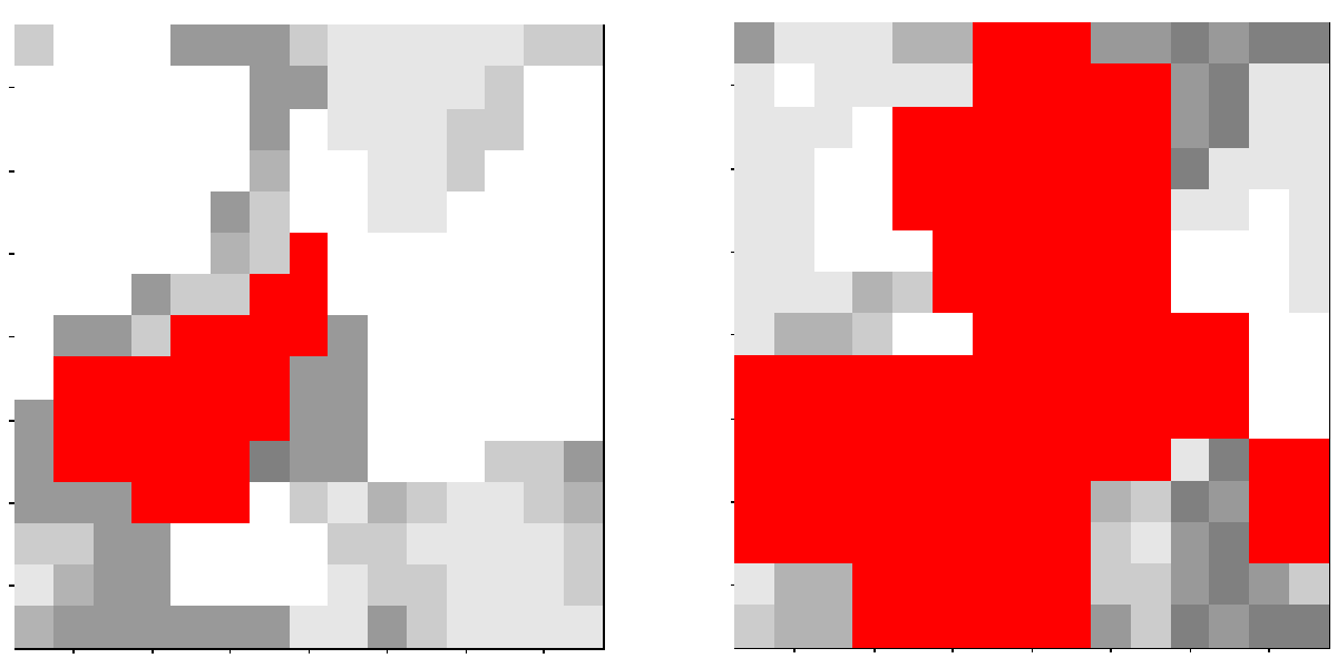
- fire events: We implemented fire events in the following way: in every year a random number determines the number of fire events within this year. This fire frequency is poisson distributed (Green 1989) with $\lambda$ as mean time between fire events. If a fire event occurs, the fire centre is chosen randomly within the simulated forest area. The fire size (equal to the number of burned patches) is described by an exponential distribution $\beta$ as mean size of the fire area related to the whole simulated forest area (Green 1989). The fire spread is modelled randomly: (i.) going from the fire centre every neighboring patch is burned, (ii.) a randomly burned patch is chosen and (iii.) again every neighboring patch is burned. This procedure is repeated until the number of the burned patches is equal to the specified fire size.
 Figure 11: Visualization of two randomly chosen fire events. The simulated area is nine hectare. The grey level indicates the amount of standing biomass. The red colour shows the fire spread.
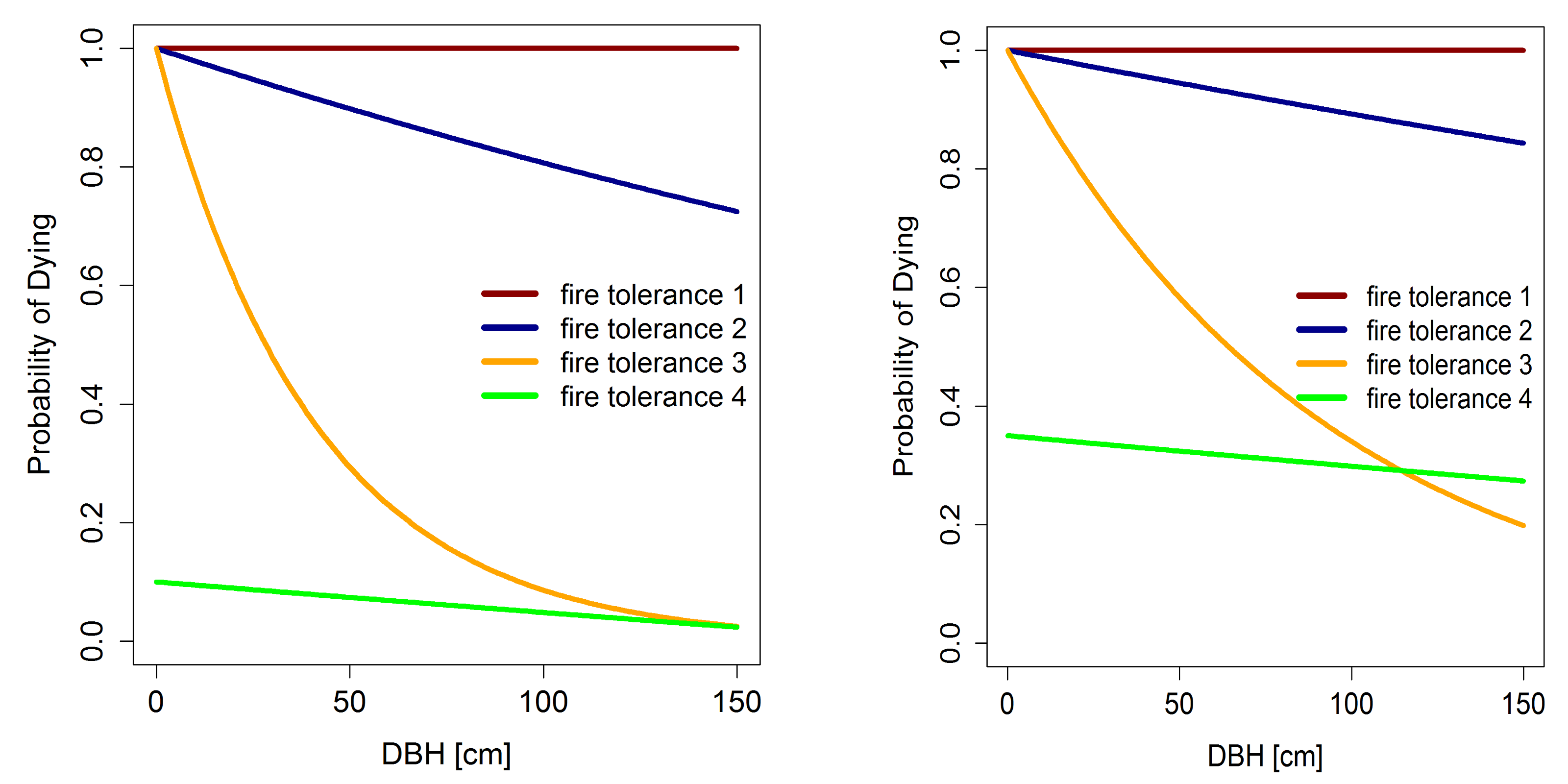
- fire tolerance of trees: According to the fire tolerance of a tree species, not every tree is burning and dying in the fire area. The probability for tree burning depends on fire tolerance of the species, on the stem diameter ($D$ $[cm]$) as a proxy of tree age and on the fire severity (Busing & Solomon 2006). We distinguish between four fire tolerance levels for tree species. Tree species of level 1 are dying in a fire, independent of stem diameter or fire severity. Tree species with a fire tolerance up to level 4 have an increasing fire-resistance. The burning probability for every tree is calculated as follows depending on the fire tolerance of the tree species (Busing & Solomon 2006):
\begin{align}
P_{F1} &= 1 \\ P_{F2} &= e^{((-(1-s_{fire}) \cdot 0.00202)-0.00053) \cdot D} \\ P_{F3} &= e^{((-(1-s_{fire}) \cdot 0.02745)-0.00255) \cdot D} \\ P_{F4} &= e^{-0.00053 \cdot D} - 0.5 - (1 - s_{fire}) \cdot 0.5 \end{align} where $s_{fire}$ (value between $0-1$) is an indicator for the severity and the type of the fire (see figure below) and $D$ is the stem diameter.
 Figure 12: Probability for tree dying after a fire event depending on stem diameter ($D$) and fire tolerance group. Left: probability of dying after a weak fire event ($s_{fire} = 0.2$). Right: probability of dying after a strong fire event ($s_{fire} = 0.7$).
Landslides
In montane forests shallow landslides can constitute a recurring natural disturbance. Disturbance by landslides differs from disturbances by falling trees or logging in the sense that all vegetation, as well as upper soil layers and seed bank are removed from the disturbed patch. Forest regeneration on landslide surfaces therefore underlies particular environmental conditions. For instance, solar radiation on recent landslide sites is high and nutrient levels of landslide soils are low (Wilcke et al. 2003). Due to this changed environmental conditions, establishment rates of trees as well as tree mortality and tree growth rates might deviate from the basic type-specific rates.
To study potential effects of landslide disturbances on the forest carbon cycle and species composition, we implemented landslides as a particular type of disturbance into the FORMIND 3.0 model. External inputs to the landslide module are the landslide frequency per hectare and year ($slidefreq$) and the distribution of landslide sizes. Landslide disturbance is implemented on the patch level, i.e. the smallest possible landslide has the size of one patch $A_{patch}$ (i.e. 20 m x 20 m) and the biggest landslides considered are for example 25 patches (1 hectare).
We implemented landslides in the following way: for each hectare and in every year a randomly drawn number determines whether a landslide occurs (probability $f_{land}$). Since the annual frequency on a per hectare basis will usually be small, we do not account for multiple landslides on one hectare in the same year. The size of the landslide is drawn from a size distribution ($s$) of landslides, rounded for the patch size $A_{patch}$. The starting location of the landslide is a random patch and the directionality of landslides is always the same. Neighbouring patches of the starting location are affected until the slide reaches the predetermined size. All trees in landslide affected patches die and are removed from the patch. Since recruiting trees in FORMIND 3.0 have a stem diameter of $D_{min}$ $[cm]$ at breast height, there is a time lag ($t_{lag}$) between the landslide event and the occurrence of the first trees on the slide surface. Based on the potential growth of trees this time lag can be estimated for the different tree types. Forest recovery then proceeds according to one of the following scenarios: undisturbed regrowth, reduced growth, reduced recruitment, increased mortality. For the justification of these scenarios, see Dislich & Huth 2012.
- Undisturbed regrowth: All type-specific parameters stay unchanged. This situation considers increased light levels after the landslide disturbance but neglects additional environmental changes.
All other scenarios describe a temporal change in type-specific traits. The underlying assumption is that the strongest change in traits occurs immediately after the landslide and traits come back to their normal level, as forest recovery proceeds after the disturbance. The parameter $r_{land}$ represents the assumed change in tree species attributes after landslide occurrence.
-
Reduced growth: FORMIND 3.0 calculates tree growth as biomass increment per year ($\Delta B$, cf. section F.3). Assuming a simple linear relation between growth reduction and "recovery status" of the disturbed site, which is expressed by the ratio of accumulated dead biomass ($B_{dead}$) to the minimum biomass in a mature patch ($B_{mat}$), the reduced biomass increment ($\Delta B_{red}$) is calculated via: \begin{align} \Delta B_{red}(B_{dead}) &= \left( r_{land} \cdot \frac{B_{dead}}{B_{mat}} + (1 - r_{land}) \right) \cdot \Delta B \end{align}
-
Reduced recruitment: The type-specific recruitment rate per hectare and year ($N_{seed}$, cf. section C) might be changed due to landslide disturbances. Like in the reduced growth scenario, we assume a linear relationship between the amount of recruitment reduction and recovery status of the patch, now expressed by the ratio of established biomass in the recovering patch ($B_{pat}$) to the minimum biomass of a mature patch ($B_{mat}$). Therefore the reduced recruitment rate ($N_{red}$) is calculated via: \begin{align} N_{red}(B_{dead}) &= \left( r_{land} \cdot \frac{B_{pat}}{B_{mat}} + (1 - r_{land}) \right) \cdot N_{seed} \end{align}
-
Increased mortality: The type-specific mortality rate ($M$) might change due to landslide disturbance (cf. section D). Again, we assume a linear relationship between the increment in mortality rate and the recovery status of the patch, represented by the ratio of established biomass in the recovering patch ($B_{pat}$) to the minimum biomass of a mature patch ($B_{mat}$). Therefore the increased mortality rate ($M_{inc}$) is calculated as: \begin{align} M_{inc}(B_{pat}) = \left( 1 + \left( r_{land} - r_{land} \cdot \frac{b_{pat}}{B_{mat}} \right) \right) \cdot M \end{align}
The choice of the parameter $r_{land}$ as well as the chosen functional relationship between changed attributes and recovery state of the successional forest is adapted according to site specific knowledge. Exemplary values for the parameters $t_{lag}$, $r_{land}$ and $f_{land}$, as well as the slide size distribution, are shown in the tables below.
Table 4: Exemplary values for the time lag parameter $t_{lag}$ (Dislich & Huth 2012).
| Type | $t_{lag}$ |
|---|---|
| pioneer species | 3 |
| mid-successional species | 5 |
| climax species | 12 |
Table 5: Exemplary values for the parameters $r_{land}$ and $f_{land}$ (Dislich & Huth 2012).
| Parameter | Value |
|---|---|
| $r_{land}$ | 0.9, 0.5 |
| $f_{land}$ | 0.02 |
Table 6: Exemplary slide size distribution $s$ (Dislich & Huth 2012).
| Landslide size [$m^2$] | Frequency |
|---|---|
| 400 | 0.30 |
| 800 | 0.26 |
| 1200 | 0.16 |
| 1600 | 0.09 |
| 2000 | 0.08 |
| 2400 | 0.03 |
| 2800 | 0.03 |
| 3200 | 0.01 |
| 3600 | 0.03 |
| 4000 | 0.005 |
| 4400 | 0.005 |
| $\geq$ 4800 | 0 |